The Geometry of the Infinite
AbstractHow to read this document
A fractal is a shape that refuses to simplify when you look closer. Where classical geometry promises that a smooth curve, magnified enough, eventually looks like a straight line, a fractal answers magnification with more structure — endlessly, and often with the same structure repeating. This single stubborn property forces us to rebuild some of our most basic intuitions: about dimension, about length and area, about what it means for a process to be "solved." It also happens to produce some of the most beautiful images mathematics has ever generated.
This document is the scientific groundwork for an application that generates art from fractal equations. The brief was deliberate: understand the field before building on it. So this is not a tutorial and not a marketing tour — it is a field guide written for rigor. It develops the mathematics properly (Hausdorff dimension, contraction mappings, complex dynamics, Lyapunov theory), it catalogues every major family with its defining equations and exact dimensions, it derives the rendering and coloring algorithms that make these objects visible, and only then does it translate all of that into a concrete software architecture for the web.
The document is organized in ten parts. Parts I–VI are the mathematics: foundations and dimension theory; iterated function systems; L-systems; complex dynamics (the Mandelbrot and Julia sets and their cousins); chaos and strange attractors; and the three-dimensional frontier. Part VII is the hinge of the whole project — the science of rendering and color, where mathematics becomes image. Part VIII covers the numerical reality of deep zooming. Part IX is the engineering blueprint: how to structure the app so that every fractal in Parts I–VI is a plug-in behind one clean interface. Part X is reference material — a master comparison table, a glossary, and sources.
Every figure here was rendered from scratch at the equations shown — no stock images — so that what you see is exactly what the mathematics produces.
Part IFoundations — What Is a Fractal?
1.1 A short history of a long idea
For most of its history, mathematics treated the pathological with suspicion. When Karl Weierstrass presented (1872) a function that is continuous everywhere yet differentiable nowhere — \(W(x)=\sum_{n=0}^{\infty} a^{n}\cos(b^{n}\pi x)\) with \(0
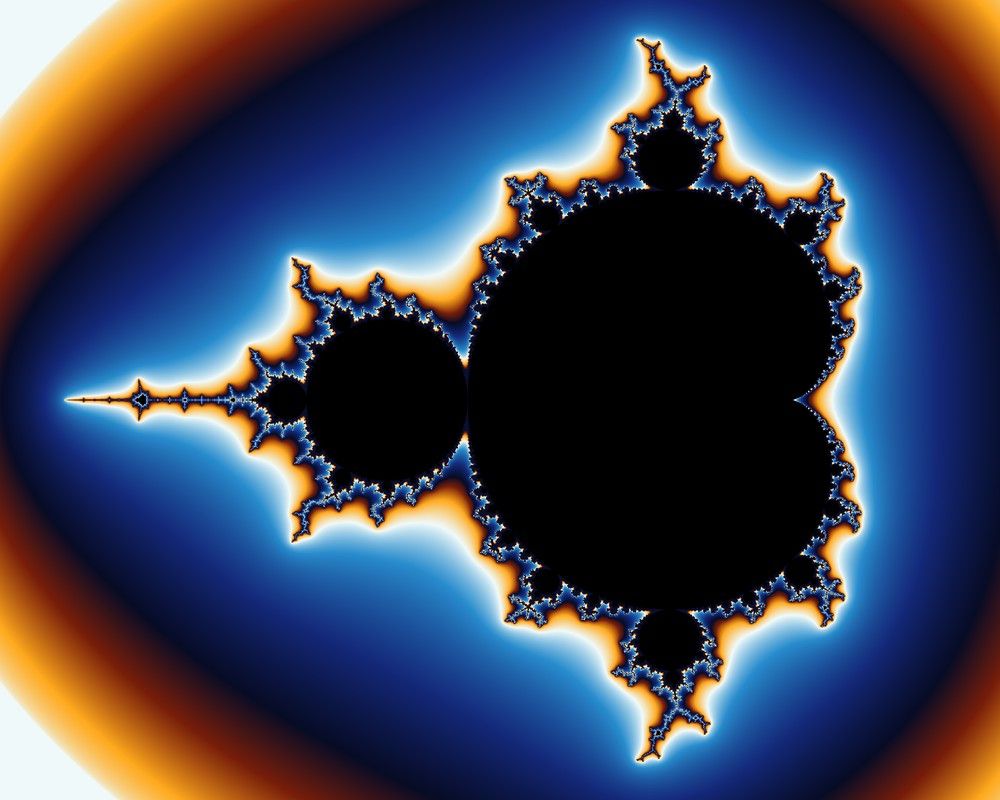
The unifying language arrived in two stages. Felix Hausdorff (1918) defined a notion of dimension that could take non-integer values, made rigorous by Abram Besicovitch. Then Benoit Mandelbrot, with access to IBM's computers, saw that these scattered monsters were not exceptions but the rule in nature — coastlines, mountains, turbulence, blood vessels, price series. In 1975 he coined fractal (from Latin fractus, "broken"), and his 1982 book The Fractal Geometry of Nature turned a museum of curiosities into a science. The set in Figure 1, which he first plotted clearly in 1980, became its emblem.
1.2 The crisis of dimension
What exactly is "broken" about a fractal is its dimension. We carry two different ideas of dimension that usually agree and, for fractals, do not.
The Lebesgue covering dimension \(\dim_T F\) is the least integer \(n\) such that every open cover of \(F\) has a refinement in which no point lies in more than \(n+1\) sets. A point has \(\dim_T=0\); a curve, \(1\); a surface, \(2\). It is always a non-negative integer and is a topological invariant.
Topological dimension counts the "obvious" degrees of freedom. But it is blind to how a set fills space as you zoom. For that we need a metric notion. The key device, due to Hausdorff, is to measure a set at a resolution \(\delta\) and watch how the measurement scales.
For \(s\ge 0\) and a set \(F\subseteq\mathbb R^n\), define the \(s\)-dimensional Hausdorff (outer) measure by first covering \(F\) by sets of diameter at most \(\delta\):
$$\mathcal H^{s}_{\delta}(F)=\inf\Big\{\textstyle\sum_{i}(\operatorname{diam}U_i)^{s} \;:\; F\subseteq\bigcup_i U_i,\ \operatorname{diam}U_i\le\delta\Big\},\qquad \mathcal H^{s}(F)=\lim_{\delta\to 0}\mathcal H^{s}_{\delta}(F).$$There is a unique critical value \(s^\star\) at which \(\mathcal H^{s}(F)\) jumps from \(+\infty\) to \(0\). That value is the Hausdorff dimension:
$$\dim_{H} F=\inf\{s\ge 0:\mathcal H^{s}(F)=0\}=\sup\{s\ge 0:\mathcal H^{s}(F)=\infty\}.$$This recovers the familiar cases (a smooth curve has \(\dim_H=1\), \(\mathcal H^1=\) its length; a disc has \(\dim_H=2\)), but it also allows a set to sit between integers. A more computable cousin replaces clever covers with a uniform grid.
Let \(N_\delta(F)\) be the number of boxes in a grid of side \(\delta\) that meet \(F\). Then
$$\dim_{B}F=\lim_{\delta\to 0}\frac{\log N_\delta(F)}{\log(1/\delta)},$$when the limit exists. In general \(\dim_{H}F\le \underline{\dim}_{B}F\le \overline{\dim}_{B}F\), and for the self-similar sets below all three coincide. Box-counting is what one actually estimates from data (and from images): plot \(\log N_\delta\) against \(\log(1/\delta)\) and measure the slope.
1.3 Self-similarity and the similarity dimension
Most "designed" fractals are built from scaled copies of themselves, and for them dimension has a beautifully simple closed form. Suppose a set is the union of \(N\) non-overlapping copies of itself, each scaled by a factor \(r<1\). Conservation of \(s\)-dimensional measure under the \(N\) maps requires \(N\,r^{\,s}=1\), giving the similarity dimension
More generally, with unequal ratios \(r_1,\dots,r_N\), the dimension \(s\) is the unique root of the Moran equation \(\sum_{i=1}^{N} r_i^{\,s}=1\). Moran's theorem (1946) guarantees that when the copies satisfy the open set condition (they do not overlap too much — formally, there is a nonempty open \(V\) with \(\bigcup_i f_i(V)\subseteq V\) and the \(f_i(V)\) disjoint), the similarity dimension equals the Hausdorff dimension. The classic values:
| Set | Copies \(N\) | Scaling \(r\) | \(\dim_H=\log N/\log(1/r)\) | \(\dim_T\) |
|---|---|---|---|---|
| Cantor middle-thirds set | 2 | 1/3 | \(\log 2/\log 3\approx 0.6309\) | 0 |
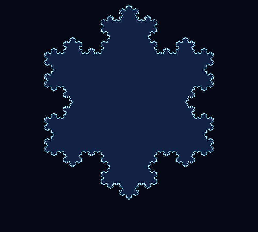
| Koch curve | 4 | 1/3 | \(\log 4/\log 3\approx 1.2619\) | 1 |
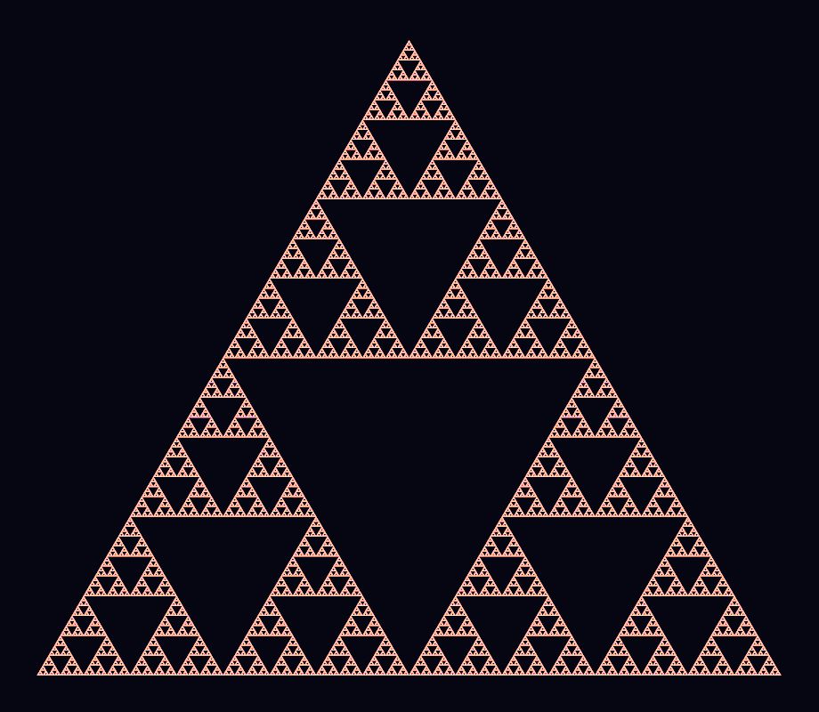
| Sierpiński triangle (gasket) | 3 | 1/2 | \(\log 3/\log 2\approx 1.5850\) | 1 |
| Sierpiński carpet | 8 | 1/3 | \(\log 8/\log 3\approx 1.8928\) | 1 |
| Menger sponge | 20 | 1/3 | \(\log 20/\log 3\approx 2.7268\) | 1 |
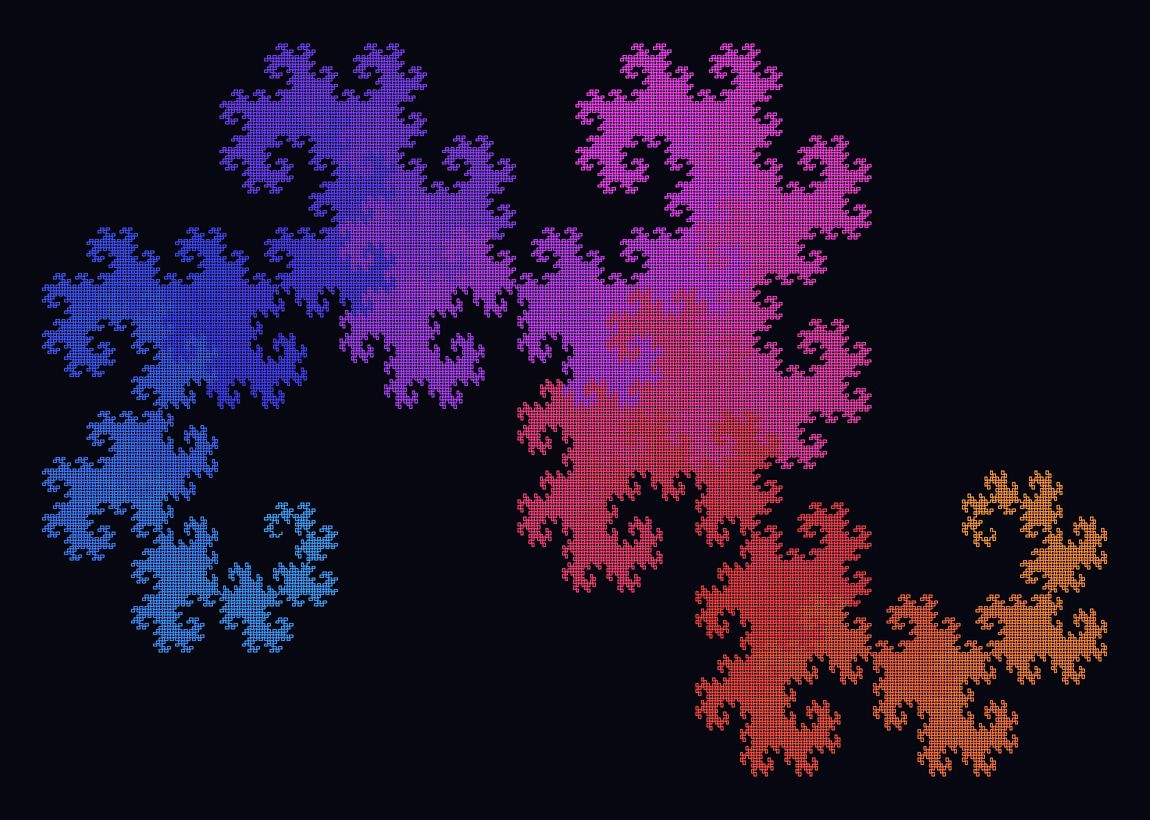
| Heighway dragon (boundary) | — | — | \(2\) (area-filling); bdry \(\approx 1.5236\) | 1 |
Each value reads as a sentence. The Cantor set, dimension \(\approx0.63\), is "more than points but less than a line." The Koch curve, \(\approx1.26\), is "more than a line but less than a plane" — it is so wrinkled that no finite length describes it, yet it is too thin to have area. The Sierpiński carpet, \(\approx1.89\), is nearly plane-filling. These are not metaphors; they are the exponents at which Hausdorff measure is finite and nonzero.
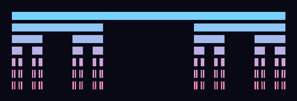
Mandelbrot's 1982 working definition was: a fractal is a set whose Hausdorff dimension strictly exceeds its topological dimension, \(\dim_H>\dim_T\). It captures the Cantor set, Koch curve, and Sierpiński sets perfectly. But it is imperfect at the edges: the image of a Peano/Hilbert space-filling curve is just a filled square (\(\dim_H=\dim_T=2\), not a fractal as a set), even though the construction is the epitome of fractal recursion. Mandelbrot himself later preferred no rigid definition, describing a fractal informally as "a rough or fragmented geometric shape that can be split into parts, each of which is (at least approximately) a reduced-size copy of the whole." For our purposes the operational definition is what matters: a fractal is an object that exhibits structure across a wide range of scales, generated by the iteration of a rule.
1.4 Kinds of self-similarity, and why nature is fractal
It is useful to distinguish three grades of self-similarity, because they map directly onto the three large algorithmic families in this guide.
- Exact self-similarity. The set is identical to scaled copies of itself (Cantor, Koch, Sierpiński). These come from iterated function systems (Part II).
- Quasi-self-similarity. Small regions resemble the whole but with distortion — the rule is not a simple rescaling. The Mandelbrot set is quasi-self-similar: tiny "baby Mandelbrots" appear throughout its boundary, slightly deformed. These come from escape-time dynamics (Part IV).
- Statistical self-similarity. Only numerical or statistical measures (like the box-counting dimension) are scale-invariant; no two pieces are literally alike. This is the self-similarity of coastlines, clouds, and Brownian motion (Part V).
The reason fractals describe nature is that nature builds by iteration under constraints — branching that minimizes transport cost (lungs, rivers, vasculature), aggregation, erosion, turbulent cascades. Mandelbrot's "How long is the coast of Britain?" (1967) made the point quantitatively: measured length grows without bound as the ruler shrinks, following a power law \(L(\delta)\propto \delta^{1-D}\) whose exponent \(D\approx1.25\) is a (box-counting) fractal dimension. Power laws and fractal dimension are two views of the same scaling symmetry — the thread that runs through every part of this document.
Part IIIterated Function Systems — the Geometry of Exact Self-Similarity
The first great fractal-generating engine is the iterated function system (IFS), introduced by John Hutchinson (1981) and developed into a practical art-and-compression tool by Michael Barnsley. The idea is to specify a fractal not by drawing it but by giving the rule of self-similarity directly: a small set of contracting maps whose combined image is the shape itself. Remarkably, this always works, and it works for a deep reason — a fixed-point theorem.
2.1 Contractions and the Banach fixed-point theorem
A map \(f:X\to X\) on a metric space \((X,d)\) is a contraction with ratio \(s<1\) if \(d\big(f(x),f(y)\big)\le s\,d(x,y)\) for all \(x,y\). Affine contractions of the plane, \(f(\mathbf x)=A\mathbf x+\mathbf b\) with \(\lVert A\rVert<1\), are the workhorses.
If \((X,d)\) is complete and \(f\) is a contraction, then \(f\) has a unique fixed point \(x^\star\), and for any starting point \(x_0\) the iterates \(f^{\circ n}(x_0)\to x^\star\) geometrically. Iteration finds the fixed point automatically.
The trick of Hutchinson was to apply this theorem not to points in the plane but to the entire space of shapes. To do that we need a metric on shapes.
Let \(\mathcal K(X)\) be the set of nonempty compact subsets of \(X\). The Hausdorff distance between \(A,B\in\mathcal K(X)\) is
$$d_H(A,B)=\max\Big\{\sup_{a\in A}\inf_{b\in B} d(a,b),\ \sup_{b\in B}\inf_{a\in A} d(a,b)\Big\}.$$Informally: the smallest \(\varepsilon\) such that \(A\) lies within \(\varepsilon\) of \(B\) and vice-versa. Crucially, if \(X\) is complete then so is \(\big(\mathcal K(X),d_H\big)\) — a fact (Blaschke's theorem) that lets us iterate on shapes.
2.2 The Hutchinson operator and the Collage Theorem
Given contractions \(f_1,\dots,f_N\) with ratios \(s_1,\dots,s_N\), define the Hutchinson operator on shapes:
\(W\) is itself a contraction on \(\big(\mathcal K(X),d_H\big)\) with ratio \(s=\max_i s_i<1\). By Banach's theorem it has a unique fixed point — a unique compact set \(\mathcal A\) with
This \(\mathcal A\) is the attractor of the IFS: the fractal. It is independent of where you start, and \(W^{\circ n}(A_0)\to\mathcal A\) for any seed \(A_0\) (a square, a dot, a photograph). This is the entire theory in one line: a fractal is the fixed point of a contraction on the space of shapes.
If a target shape \(T\) can be approximately tiled by transformed copies of itself, i.e. \(d_H\big(T,\bigcup_i f_i(T)\big)\le \varepsilon\), then the attractor \(\mathcal A\) of \(\{f_i\}\) satisfies \(d_H(T,\mathcal A)\le \varepsilon/(1-s)\). In words: to model a shape as a fractal, find maps whose collage covers it. This is the basis of fractal image compression and of designing custom IFS art — you reverse-engineer the maps from the picture you want.
2.3 Two ways to draw an IFS
Deterministic. Start with any set, apply \(W\) repeatedly, watch it converge. Accurate but expensive — the number of pieces multiplies by \(N\) each step.
The Chaos Game (random iteration). Far cheaper and the method behind most IFS art. Pick a point \(x_0\); then repeatedly choose a map \(f_i\) at random (with probabilities \(p_i\)) and set \(x_{k+1}=f_i(x_k)\). After discarding a short transient, the orbit \(\{x_k\}\) densely samples the attractor almost surely. The reason is ergodic: the random iteration is a Markov process whose invariant measure is supported exactly on \(\mathcal A\). Choosing \(p_i\propto |\det A_i|\) (each map's area contraction) equalizes the visiting density, which is what makes renders look evenly exposed.
2.4 A catalogue of affine fractals
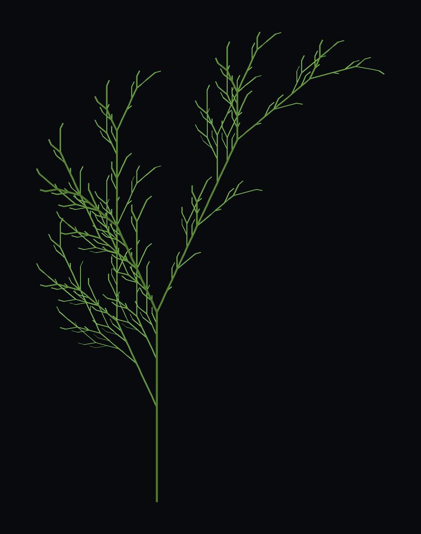
Every IFS fractal is just a table of affine maps \(f_i(\mathbf x)=A_i\mathbf x+\mathbf b_i\). The most celebrated is Barnsley's fern, whose four maps encode stem, successively smaller fronds, and the curl of the leaf.

\(f_i\!\left(\begin{smallmatrix}x\\y\end{smallmatrix}\right)=\left(\begin{smallmatrix}a&b\\c&d\end{smallmatrix}\right)\!\left(\begin{smallmatrix}x\\y\end{smallmatrix}\right)+\left(\begin{smallmatrix}e\\f\end{smallmatrix}\right)\), with rows \((a,b,c,d,e,f,p)\):
| map | a | b | c | d | e | f | p | role |
|---|---|---|---|---|---|---|---|---|
| \(f_1\) | 0 | 0 | 0 | 0.16 | 0 | 0 | 0.01 | stem |
| \(f_2\) | 0.85 | 0.04 | −0.04 | 0.85 | 0 | 1.60 | 0.85 | successive fronds |
| \(f_3\) | 0.20 | −0.26 | 0.23 | 0.22 | 0 | 1.60 | 0.07 | left leaflet |
| \(f_4\) | −0.15 | 0.28 | 0.26 | 0.24 | 0 | 0.44 | 0.07 | right leaflet |
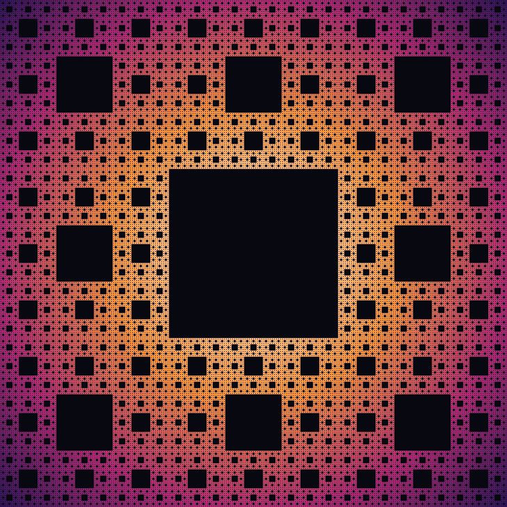
Other members worth supporting in software, all specified by the same affine-table format: the Cantor dust (Cantor set in 2D), the Lévy C curve, the Koch curve and its variants, the Pythagoras tree (two maps, a square branching into two scaled-and-rotated squares), the McWorter pentigree, and the space-filling Peano and Hilbert curves (limits of curve sequences; useful both as art and as locality-preserving orderings for the tiled renderer in Part IX). Because they share one data shape — a list of maps with probabilities — a single IFS engine renders all of them, which is exactly how we will architect them in the application.
Part IIIL-systems — the Grammars of Growth
Where an IFS specifies a fractal by geometric maps, an L-system specifies one by language — a rewriting grammar applied in parallel. Introduced by the biologist Aristid Lindenmayer (1968) to model the growth of filamentous algae, L-systems became, through Lindenmayer and Prusinkiewicz's The Algorithmic Beauty of Plants, the standard way to generate botanical fractals and the branching structures that IFS handles awkwardly.
3.1 Formal definition
A deterministic, context-free L-system is a triple \(G=(V,\omega,P)\): an alphabet \(V\); an axiom \(\omega\in V^{+}\) (the starting string); and a set of production rules \(P\subseteq V\times V^{*}\), one per symbol. A derivation step rewrites every symbol simultaneously by its rule (symbols with no rule map to themselves). Iterating from \(\omega\) yields a sequence of ever-longer strings.
The defining contrast with a Chomsky grammar is parallel rewriting: all symbols are replaced at once, mirroring simultaneous cell division in a growing organism. This single change is what makes L-systems generate self-similar structure rather than parse it.
3.2 Turtle interpretation
A string becomes a drawing through turtle graphics. A virtual turtle with state \((x,y,\alpha)\) reads the string symbol by symbol:
F— move forward one step, drawing a segment;f— move without drawing.+/−— turn left / right by a fixed angle \(\delta\).[/]— push / pop the turtle state on a stack. These brackets are what allow branching: descend into a sub-branch, then return exactly to the fork.
The bracket mechanism turns a one-dimensional string into a tree, and the parallel rewriting makes each branch a smaller copy of the whole — exact self-similarity emerging from grammar.
3.3 Worked examples
Koch curve. \(V=\{F,+,-\}\), axiom \(F\), rule \(F\to F+F--F+F\), angle \(\delta=60^\circ\). Each rewrite replaces every segment by the four-segment Koch generator — the same attractor as the IFS of Figure 3, reached by a different engine.
A plant. The bracketed system below grows the structure in Figure 8:
axiom:  X
rules:  X → F+[[X]-X]-F[-FX]+X
        F → FF
angle:  δ = 25°
Here X is a non-drawing "apex" symbol that controls branching while F→FF elongates existing stems each generation — so the plant simultaneously extends and sprouts, exactly as a meristem does.
3.4 Extensions you will want in software
- Stochastic L-systems. Attach probabilities to multiple rules for one symbol, \(p_1\!:F\to\ldots\ \mid\ p_2\!:F\to\ldots\), so each plant grown from the same grammar is unique — essential for natural-looking variety and for art that is generative rather than fixed.
- Parametric L-systems. Symbols carry parameters, \(F(\ell)\), with rules that compute on them, e.g. \(F(\ell)\to F(\ell/2)\). This encodes continuous growth, tapering, elapsed time, and physical quantities.
- Context-sensitive (IL) systems. A rule can depend on a symbol's neighbors, modeling signals propagating through the organism (e.g. a flowering hormone sweeping up a stem).
- 3D turtle. Add roll/pitch/yaw operators (
&,^,\\,/) and a full orientation frame to grow trees in space — directly relevant to Part VI.
For the application, an L-system module needs only: an alphabet-and-rules editor, a parallel-rewrite engine with a generation cap, and a turtle interpreter (2D and 3D) that emits line segments or cylinders. The same emitted-geometry buffer then flows into the renderer used by every other family.
Part IVComplex Dynamics — the Escape-Time Fractals
The richest fractals come not from a fixed geometric rule but from iterating a function on the complex plane and asking a single question at every point: does the orbit stay bounded, or fly to infinity? The boundary between "bounded" and "escapes" is, generically, a fractal — and for the quadratic family it is the Mandelbrot set and its Julia sets, the objects that made fractals famous. This is the theory of complex dynamics, founded by Fatou and Julia and transformed by Douady, Hubbard, and others.
4.1 Iteration, orbits, and the dichotomy of stability
Fix \(c\in\mathbb C\) and study the quadratic map
A fixed point satisfies \(z^\star=f_c(z^\star)\); its multiplier \(\lambda=f_c'(z^\star)=2z^\star\) governs local behavior. The orbit is drawn toward \(z^\star\) when \(|\lambda|<1\) (attracting), pushed away when \(|\lambda|>1\) (repelling), and delicately balanced when \(|\lambda|=1\) (neutral: parabolic if \(\lambda\) is a root of unity, otherwise Siegel or Cremer). The same classification applies to periodic points via the multiplier of the iterate. This local picture organizes everything that follows.
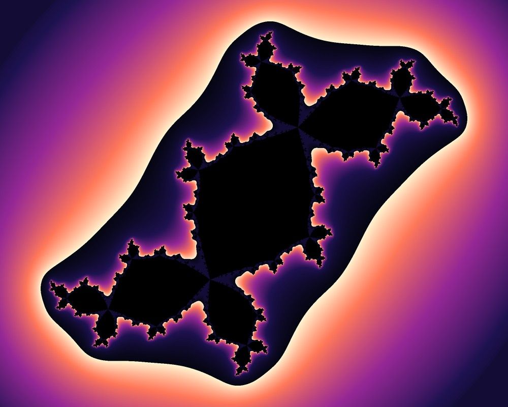
The filled Julia set of \(f_c\) is the set of points with bounded orbit,
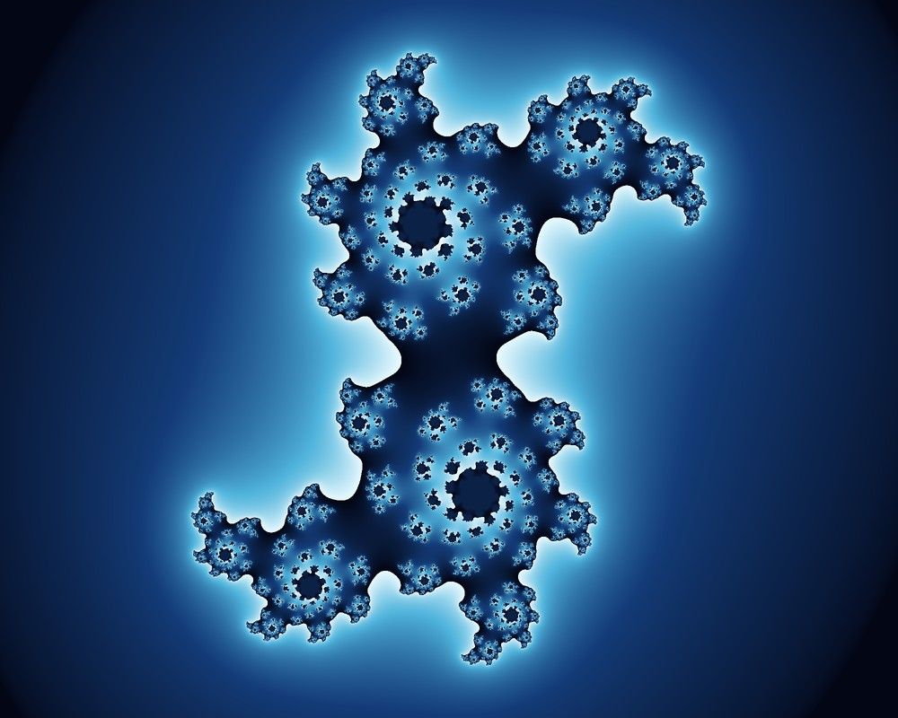
$$K_c=\{z\in\mathbb C:\ \{f_c^{\circ n}(z)\}_{n\ge0}\ \text{is bounded}\}.$$The Julia set is its boundary \(J_c=\partial K_c\); the Fatou set is the complement \(\mathbb C\setminus J_c\), where dynamics is stable (nearby orbits stay nearby). \(J_c\) is the locus of sensitive dependence — chaos lives there.
The Julia set has striking structural properties, each useful in rendering: it is nonempty, compact, and perfect (no isolated points); it is completely invariant, \(f_c^{-1}(J_c)=J_c=f_c(J_c)\); it equals the closure of the repelling periodic points; and it is the boundary of the basin of attraction of \(\infty\). That last fact is exactly why the escape-time algorithm (Part VII), which colors by speed of escape, draws \(J_c\) "for free."
4.2 The Fundamental Dichotomy
The function \(f_c\) has a single critical point, \(z=0\) (where \(f_c'=0\)). The fate of that one point decides the global topology of the whole Julia set — a theorem of Fatou and Julia of astonishing economy.
For \(f_c(z)=z^2+c\), exactly one of two cases holds:
(i) if the critical orbit \(\{f_c^{\circ n}(0)\}\) is bounded, then \(J_c\) (and \(K_c\)) is connected;
(ii) if the critical orbit \(\to\infty\), then \(J_c=K_c\) is totally disconnected — a Cantor set of dust, with empty interior.
Sketch. The basin of \(\infty\) is, near \(\infty\), conformally a disk. Pulling it back by \(f_c\) either preserves connectivity (when no critical point lies in the escaping region, case i) or splits each pre-image into two, generating at the limit the binary Cantor structure of case (ii). The critical point is the only obstruction to taking single-valued inverse branches, so its orbit is decisive.
4.3 The Mandelbrot set as a map of all Julia sets
The dichotomy makes the parameter \(c\) the natural variable to study. Collect every \(c\) that gives a connected Julia set:
$$M=\{c\in\mathbb C:\ J_c\ \text{is connected}\}=\{c\in\mathbb C:\ \text{the orbit of }0\ \text{under }f_c\ \text{is bounded}\}.$$
The two descriptions agree by Theorem 4.2. Thus \(M\) is simultaneously a catalogue (each point is one Julia set's "connectedness verdict") and a dynamical object in its own right. Picking \(c\) on or near \(M\)'s features yields the most beautiful Julia sets — the basis of the "linked Julia" tool we will build.
To compute \(M\) we need to know when to stop iterating. The answer is a clean lemma with the escape radius \(R=2\).
If at some step \(|z_n|>2\) and \(|z_n|\ge|c|\), the orbit diverges to \(\infty\). Hence \(M\subseteq\{|c|\le2\}\), and "\(|z|>2\)" is a sound bailout test.
Proof. Suppose \(|z_n|\ge|c|\) and \(|z_n|=2+\varepsilon\), \(\varepsilon>0\). Then
$$|z_{n+1}|=|z_n^2+c|\ge|z_n|^2-|c|\ge|z_n|^2-|z_n|=|z_n|\,(|z_n|-1)\ge|z_n|\,(1+\varepsilon).$$So each step multiplies the modulus by at least \(1+\varepsilon>1\); the orbit grows geometrically and escapes. (For \(c\in M\), \(0\) never escapes, and one checks \(|c|\le2\) directly.) \(\;\blacksquare\)
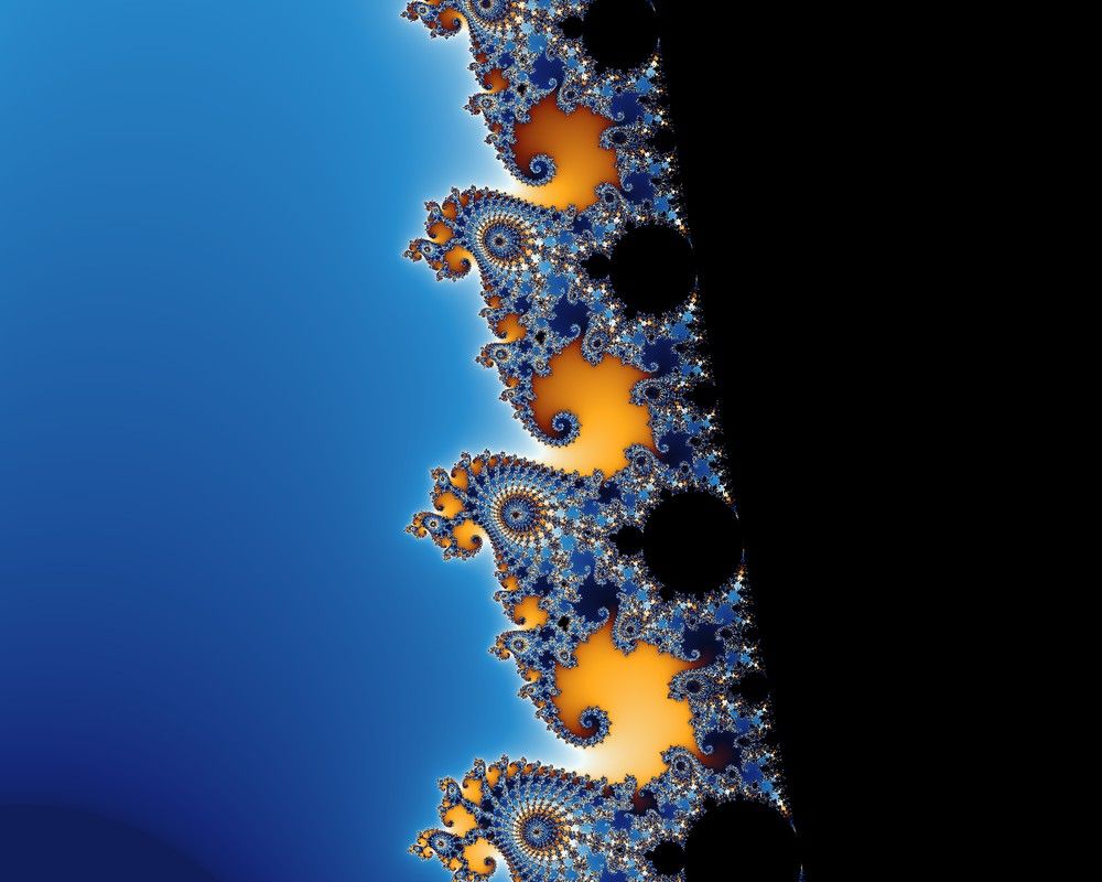
Everything visible in Figure 1 — the colored exterior — is a graph of how many iterations a point needs to cross \(|z|=2\). Part VII turns that integer into a continuous, paintable quantity.
4.4 The anatomy of \(M\)
The Mandelbrot set is not a blob; it is an intricately organized hierarchy. Its interior is (conjecturally, all of it) a union of hyperbolic components — open regions where \(f_c\) has an attracting cycle of some period. The largest is the main cardioid.
The set of \(c\) for which \(f_c\) has an attracting fixed point is the cardioid traced by
$$c(\mu)=\frac{\mu}{2}-\frac{\mu^{2}}{4},\qquad |\mu|\le 1 ,$$with boundary \(\mu=e^{i\theta}\). Why: a fixed point obeys \(z^\star=z^{\star2}+c\) with multiplier \(\mu=2z^\star\); solving \(z^\star=\mu/2\) and substituting gives \(c=z^\star-z^{\star2}=\mu/2-\mu^2/4\). The point is attracting exactly when \(|\mu|<1\), i.e. inside the cardioid.
Tangent to the cardioid at \(c=-\tfrac34\) (where \(\mu=-1\)) is the period-2 bulb, the disk \(|c+1|<\tfrac14\) — the set of \(c\) with an attracting 2-cycle. Off each hyperbolic component sprout infinitely many smaller bulbs, one for every rational internal angle \(p/q\in\mathbb Q/\mathbb Z\): the bulb at angle \(p/q\) is a period-\(q\) component, and the "antenna" growing from it has exactly \(q\) spokes (Douady). The bulbs are ordered around the cardioid by the Farey/Stern–Brocot arithmetic of their angles — between the \(p_1/q_1\) and \(p_2/q_2\) bulbs, the largest one in between sits at the Farey mediant \((p_1+p_2)/(q_1+q_2)\). The Mandelbrot set is, in this sense, a geometric encoding of the rationals.
Two further landmarks matter for both theory and art:
- Misiurewicz points — parameters where the critical orbit is strictly pre-periodic. They sit at the tips of antennae and the centers of spirals, and Tan Lei (1990) proved \(M\) is asymptotically self-similar there, looking locally like the corresponding Julia set. These are the most rewarding places to zoom.
- The Feigenbaum point \(c\approx-1.4011552\) — the accumulation of the period-doubling cascade \(1\!\to\!2\!\to\!4\!\to\!\cdots\) along the real axis, governed by the universal Feigenbaum constant \(\delta\approx4.6692\). The same cascade and constant appear in the logistic map of Part V — a deep unity between the real and complex pictures.
(Douady–Hubbard, 1982) \(M\) is connected. The proof exhibits an explicit conformal isomorphism \(\Phi:\mathbb C\setminus M\to\mathbb C\setminus\overline{\mathbb D}\) onto the exterior of the unit disk (via Böttcher coordinates of \(f_c\)); the pre-images of circles and rays are the equipotentials and external rays that the coloring of Figure 1 makes visible.
(Shishikura, 1991) The boundary \(\partial M\) has Hausdorff dimension exactly \(2\) — maximal roughness — even though \(M\) has finite area \(\approx1.5065\). This is why anti-aliasing the Mandelbrot boundary is genuinely hard (Part VII): detail exists at every scale, everywhere on the boundary.
(MLC, open) The conjecture that \(M\) is locally connected would, by Douady–Hubbard's "pinched-disk" model, give a complete combinatorial description of \(M\) by external angles. Yoccoz proved it at all finitely-renormalizable points; the general case remains one of the central open problems of dynamics.
4.5 Variants and cousins — one engine, many worlds
The escape-time recipe — iterate, test a bailout, color by the rate — generalizes far beyond \(z^2+c\). Each variant below is a small change to the iteration formula, which is exactly why a single configurable kernel can render them all.
Multibrots \(z^{d}+c\)
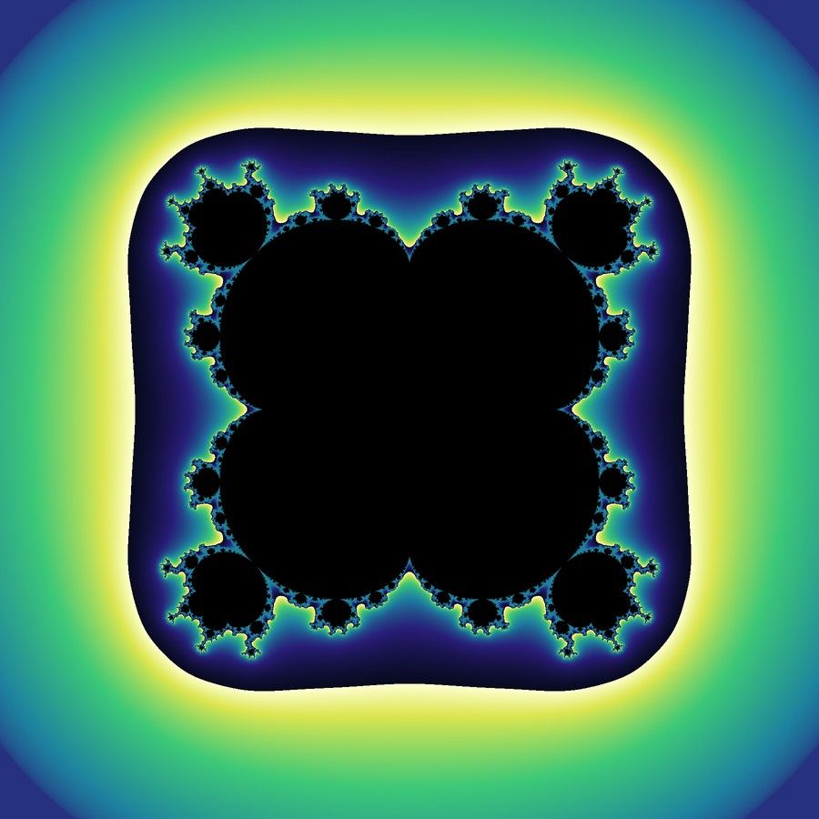
Raising the power gives \(f_c(z)=z^{d}+c\). The resulting "multibrot" has \((d-1)\)-fold rotational symmetry and \(d-1\) primary bulbs; the case \(d=2\) is Mandelbrot. Non-integer and negative \(d\) produce further families.
The Burning Ship — when analyticity breaks
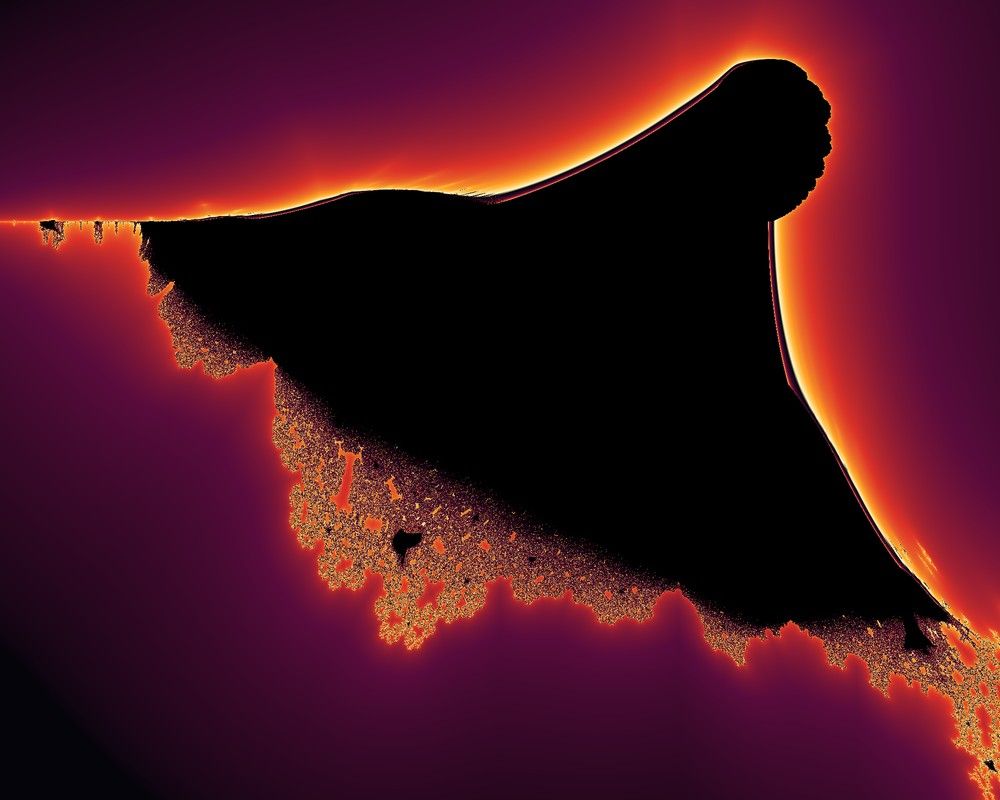
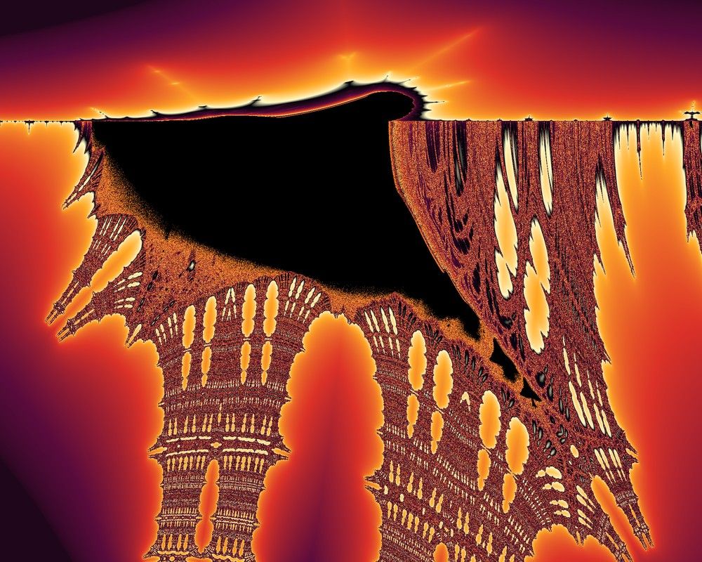
Take absolute values of the real and imaginary parts before squaring (Michelitsch & Rössler, 1992):
The folds \(|\cdot|\) make the map non-holomorphic, so the elegant Fatou–Julia theory does not apply — there is no clean Julia/Mandelbrot conjugacy. Yet the escape-time algorithm is indifferent to analyticity, and the result is one of the most evocative fractals known: a fleet of "ships" wreathed in flame-like detail.
Newton fractals — chaos from root-finding
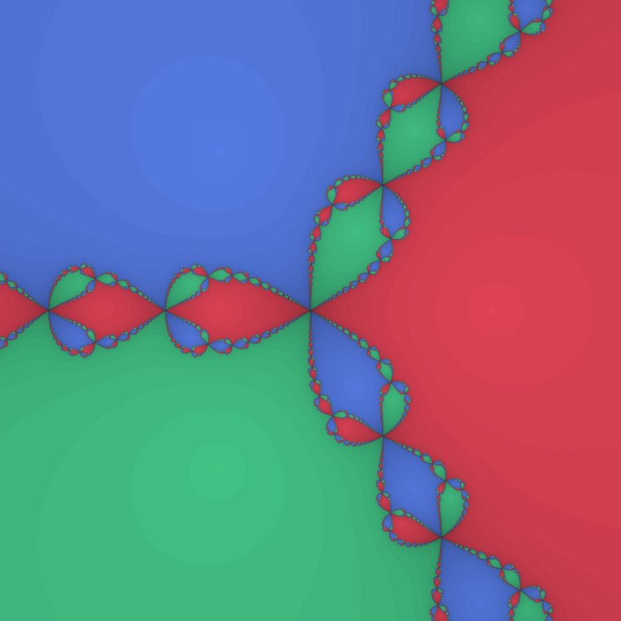
Apply Newton's method to a polynomial \(p\): iterate \(z_{n+1}=z_n-\dfrac{p(z_n)}{p'(z_n)}\). Each root has a basin of attraction; coloring each point by which root it converges to (and shading by how fast) reveals a fractal boundary between basins — itself the Julia set of the (rational) Newton map. For \(p(z)=z^3-1\), the three cube roots of unity give three interwoven basins meeting along a curve that is locally identical everywhere.
Lyapunov fractals — the order–chaos atlas
A different escape-time idea (Markus & Hess). Drive the logistic map \(x_{n+1}=r_n x_n(1-x_n)\) with a parameter \(r_n\) that cycles through a fixed periodic sequence of two values \(a,b\) (e.g. ABAB…), and at each pixel \((a,b)\) compute the Lyapunov exponent
Where \(\lambda<0\) the dynamics is stable/periodic (ordered); where \(\lambda>0\) it is chaotic. Coloring by the sign and magnitude of \(\lambda\) maps the entire landscape of order and chaos.
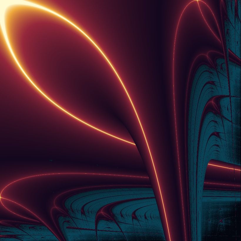
AB. Golden regions are stable (\(\lambda<0\)); dark teal is chaotic (\(\lambda>0\)). The smooth, almost organic "swallows" are the boundaries between order and chaos — a portrait of the logistic map's bifurcation structure in two dimensions.Further escape-time families to include in software, all minor edits to the kernel: Nova (a relaxed Newton iteration \(z\mapsto z-R\,p(z)/p'(z)+c\) blending Newton detail with Mandelbrot-like parameter structure); Phoenix (a second-order recurrence \(z_{n+1}=z_n^{2}+c+p\,z_{n-1}\) that remembers its previous value); Magnet fractals (from statistical-mechanics renormalization maps); and arbitrary user-entered formulas \(z\mapsto F(z,c)\) — the ultimate generalization, discussed in Part IX.
Part VChaos, Strange Attractors & Random Fractals
Fractals and chaos are two faces of one phenomenon. A chaotic dynamical system folds and stretches its state space so thoroughly that long trajectories settle onto a set of fractional dimension — a strange attractor. Here the fractal is not designed (as in an IFS) or implicit in a boundary (as in \(M\)); it is the very shape of the system's destiny.
5.1 Sensitive dependence and Lyapunov exponents
A system is chaotic when nearby trajectories separate exponentially: an initial error \(\delta_0\) grows like \(\delta(t)\approx\delta_0 e^{\lambda t}\) with Lyapunov exponent \(\lambda>0\). Positive \(\lambda\) is the precise meaning of "the butterfly effect" — deterministic yet unpredictable. The canonical 1D example is the logistic map \(x_{n+1}=r\,x_n(1-x_n)\): as \(r\) increases it undergoes a period-doubling cascade \(2\to4\to8\to\cdots\) accumulating at \(r_\infty\approx3.5699\), beyond which it is chaotic. The cascade's geometric rate is the universal Feigenbaum constant \(\delta\approx4.66920\) — universal because the same number governs period-doubling in vast classes of systems, including the real slice of the Mandelbrot set (Part IV). Chaos has constants.
5.2 Strange attractors
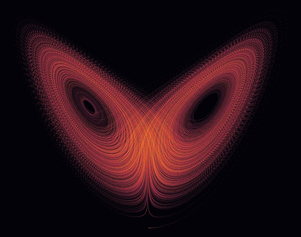
In continuous time, the simplest strange attractor is Lorenz's (1963), distilled from atmospheric convection:
with the classic \(\sigma=10,\ \rho=28,\ \beta=\tfrac83\). Trajectories never repeat yet never leave a bounded "butterfly," whose correlation dimension is \(\approx2.06\): more than a surface, less than a volume.
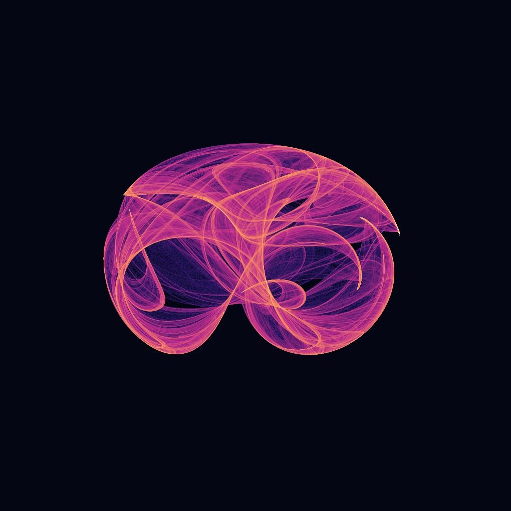
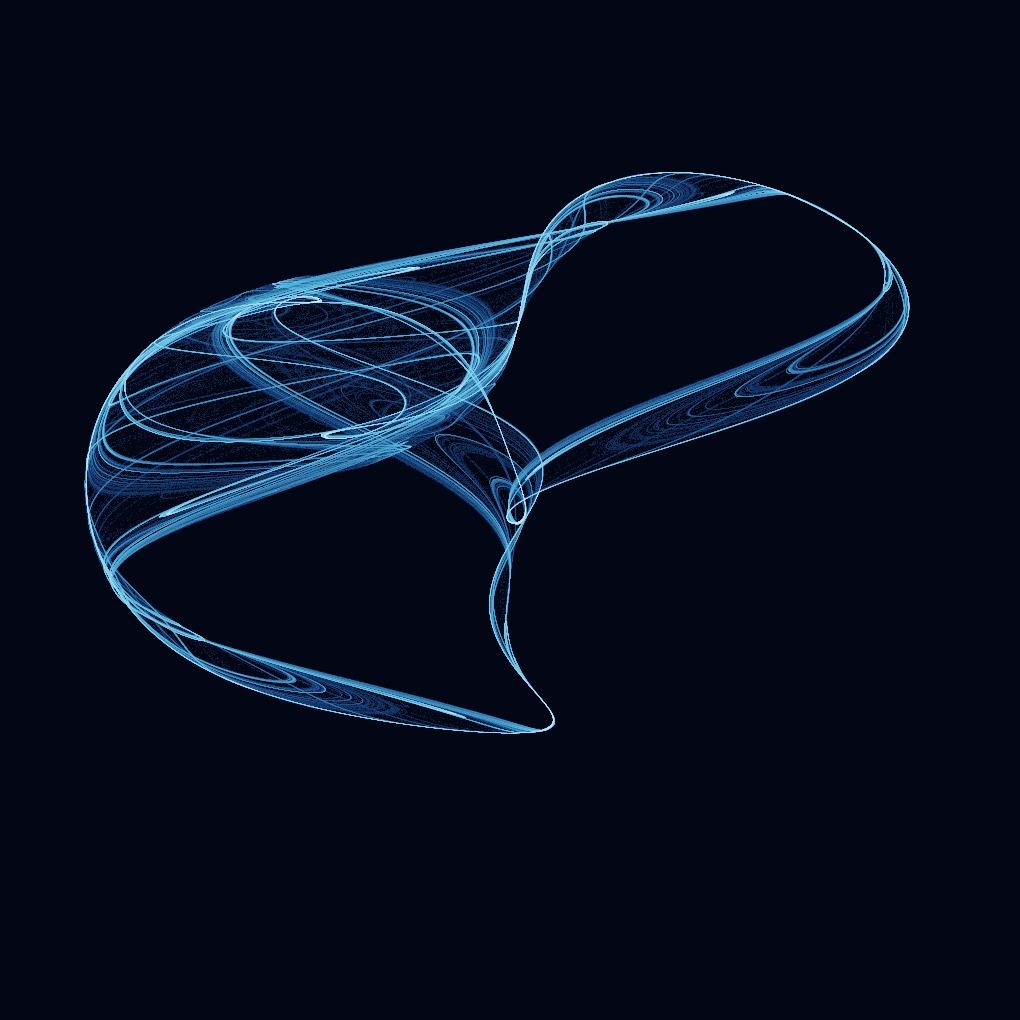
Discrete-time maps give equally rich attractors and are trivial to iterate, making them ideal for an art tool. The Hénon map \((x,y)\mapsto(1-ax^2+y,\ bx)\) with \(a=1.4,b=0.3\) has a Cantor-like cross-section (dimension \(\approx1.26\)). The Clifford and de Jong attractors are families tuned by four parameters each:
5.3 Measuring an attractor's dimension
For sets defined by orbits rather than rules, two operational dimensions dominate. The correlation dimension \(\nu\) (Grassberger–Procaccia) reads the power law in the correlation sum \(C(r)\sim r^{\nu}\), where \(C(r)\) counts pairs of orbit points within distance \(r\) — cheap to estimate from data. The Kaplan–Yorke (Lyapunov) dimension ties dimension directly to the exponents:
where the \(\lambda_i\) are ordered \(\lambda_1\ge\lambda_2\ge\cdots\) and \(k\) is the largest index for which \(\lambda_1+\cdots+\lambda_k\ge0\). It expresses a beautiful idea: the attractor's dimension is set by the balance between stretching (positive exponents) and the first contracting direction that reins it in.
5.4 Random fractals — the textures of nature
Determinism is optional. Many natural fractals are statistically self-similar, and they are indispensable for art that needs clouds, terrain, and organic noise.
- Brownian motion. The graph of a 1D Brownian path has Hausdorff dimension \(\tfrac32\); its planar trail has dimension \(2\). It is the prototype of a random fractal.
- Fractional Brownian motion (fBm). Parameterized by the Hurst exponent \(H\in(0,1)\): increments are positively correlated for \(H>\tfrac12\) (smooth, persistent) and anti-correlated for \(H<\tfrac12\) (rough). The graph has dimension \(2-H\) and a power-spectral density \(S(f)\propto f^{-(2H+1)}\) — "\(1/f^{\beta}\) noise." Tuning \(H\) is tuning roughness.
- Synthesis algorithms. Midpoint displacement / diamond–square generate fBm-like terrain by recursively perturbing midpoints; spectral synthesis shapes white noise in the Fourier domain by \(1/f^{\beta}\); Perlin and simplex noise (and their fractal sums, "fBm noise") are the gradient-noise workhorses of procedural graphics.
- Diffusion-limited aggregation (DLA). Particles random-walk until they stick to a growing cluster, producing branching, coral-like fractals of dimension \(\approx1.71\) in the plane — the model behind lightning, mineral dendrites, and electrodeposition.
For the application these belong to a "stochastic" family: seedable pseudo-random generators (so a piece is reproducible), an octave-summed noise module, and a terrain/landscape mode that height-maps fBm into shaded relief. Reproducibility via explicit seeds is the bridge between "random" and "art you can recreate and refine."
Part VIInto Three Dimensions — Quaternions, the Mandelbulb & the Mandelbox
An obvious dream is a 3D Mandelbrot set. It runs into an algebraic wall: there is no three-dimensional number system with the field properties of \(\mathbb C\) (a theorem ultimately rooted in Frobenius's classification of division algebras). The resolution is to go to four dimensions, or to invent a non-associative "number" in three — and both routes produce spectacular objects.
6.1 Quaternion Julia sets
The quaternions \(\mathbb H=\{a+bi+cj+dk\}\) are a genuine (non-commutative) division algebra, so \(q\mapsto q^{2}+c\) makes perfect sense for \(q,c\in\mathbb H\). The filled Julia set lives in \(\mathbb R^4\); we view a 3D slice (fixing one coordinate). These quaternion Julia sets (Norton, 1982) are smooth, glassy 4D solids — mathematically clean but visually a little austere, because the squaring map is "too symmetric."
6.2 The Mandelbulb — a triplex power
Daniel White and Paul Nylander (2009) abandoned algebraic rigor for visual richness. They defined a non-associative "triplex" power directly in spherical coordinates: writing \((x,y,z)\) as \(r=\sqrt{x^2+y^2+z^2}\), \(\theta=\operatorname{atan2}\!\big(\sqrt{x^2+y^2},\,z\big)\), \(\varphi=\operatorname{atan2}(y,x)\), the "\(n\)-th power" is
It multiplies radii and multiplies both angles — a direct lift of "square the modulus, double the argument" to the sphere. The power \(n=8\) became iconic: it produces the Mandelbulb, a bulbous, organic solid riddled with whorls and craters. It is not a true analytic Mandelbrot analogue (there is none), but it is bottomlessly self-similar and breathtaking — exactly the kind of object an art tool should reach for.
6.3 The Mandelbox — folding space
Tom Lowe (2010) built a different 3D fractal from piecewise-linear folds rather than powers. Each iteration applies, to a point \(\mathbf v\) (starting at \(\mathbf c\)):
- Box fold: for each component, if it exceeds \(1\) reflect it as \(2-v\); if below \(-1\), as \(-2-v\) (fold the point back into \([-1,1]^3\)).
- Ball fold: with radii \(r_{\min}
- Scale & translate: \(\mathbf v\leftarrow s\,\mathbf v+\mathbf c\), with a signed scale \(s\) (e.g. \(-1.5\) to \(3\)).
The result is an endless cubic, architectural lattice — corridors, towers, and rooms within rooms — utterly unlike the organic Mandelbulb. Hybridizing folds and powers across iterations (as tools like Mandelbulber and Mandelbulb 3D do) opens a combinatorial universe of forms.
6.4 Rendering 3D fractals — distance-estimated ray marching
These solids have no surface mesh, so we render them by sphere tracing: shoot a ray per pixel and step along it by a safe distance — the distance estimator (DE), a lower bound on the distance to the fractal surface. The escape-time DE generalizes the 2D formula of Part VII by carrying a scalar running derivative \(dr\) alongside the orbit. For a power-\(n\) bulb:
For the Mandelbox, \(dr\) is propagated through the folds (each fold has derivative \(\pm1\)) and the scale (multiply \(dr\) by \(|s|\)), giving \(\mathrm{DE}=|\mathbf v|/dr\). The render loop is then:
for each pixel:
  p = camera ray origin;  t = 0
  repeat:
    d = DE(p + t·dir)          // safe step toward surface
    t += d
  until d < ε  or  t > t_max
  if hit:
    n = normalize(∇ DE)        // surface normal by finite differences
    shade with lambert + soft shadow (DE along light ray)
              + ambient occlusion (from step count / iteration count)
              + orbit-trap or iteration-based color
Surface normals come from the gradient of the DE field (four extra DE evaluations); ambient occlusion falls out almost for free from how many steps the march took (crevices need more steps); soft shadows come from the minimum DE encountered along a ray to the light. Coloring reuses the orbit-trap and iteration-count ideas of Part VII applied at the hit point. This single ray-marching kernel renders Mandelbulb, Mandelbox, quaternion Julia, 3D IFS (Menger sponge, Sierpiński tetrahedron via folding DEs), and hybrids — another argument for the unified, plug-in kernel architecture of Part IX. On the web it maps naturally onto a WebGL/WebGPU fragment-or-compute shader, one ray per invocation.
Part VIIThe Science of Rendering & Color — Where Mathematics Becomes Art
This is the part the application lives or dies by. A fractal is an infinitely detailed mathematical set; an image is a finite grid of colored pixels. The map between them — how we turn iteration data into color — is not a cosmetic afterthought. It is where most of the beauty actually comes from. Two renders of the identical Mandelbrot set can look like a muddy textbook diagram or like stained glass, depending entirely on the algorithms in this part.
7.1 The escape-time algorithm, precisely
For each pixel, map it to a complex parameter \(c\) (or starting point \(z_0\)), iterate, and record when \(|z|\) crosses the bailout radius \(R\):
for each pixel → c:
  z = 0;  n = 0
  while n < maxIter and |z|² ≤ R²:
    z = z² + c
    n += 1
  if n == maxIter:  color = INTERIOR        // never escaped
  else:             color = f(n, z, …)      // escaped at step n
Three facts shape quality. (1) Use \(|z|^2\le R^2\), never a square root, in the hot loop. (2) Choose \(R\) large (e.g. \(2^{8}\)–\(2^{18}\)), not the minimal \(2\): smooth coloring (next) needs headroom, and a big \(R\) barely costs iterations because escape is super-exponential. (3) The interior — points that never escape — is the hard part: with a finite maxIter we can only ever say "hasn't escaped yet."
For points truly inside \(M\), iterating to maxIter is wasted work and dominates cost in zoomed views. Two classic accelerations: periodicity (cycle) detection — if the orbit revisits a previous value within tolerance, it is trapped in an attracting cycle, so mark it interior and stop (Floyd/Brent cycle detection, or compare against a slowly-updated reference); and the cardioid/bulb test — algebraically exclude the main cardioid and period-2 disk before iterating at all. Both are essential for interactive frame-rates.
7.2 Smooth (continuous) coloring — killing the bands
Coloring by the integer \(n\) produces ugly concentric bands (every pixel escaping at step \(n\) gets one flat color). The fix is to compute a fractional iteration count. The justification is the escape-time potential (Green's function), which for the family \(z\mapsto z^{P}+c\) is
a smooth function vanishing on the set and increasing outward (its level sets are the equipotentials seen as color contours). The key observation: once \(|z|\) is large, one more iteration nearly \(P\)-multiplies \(\ln|z|\), so \(\ln|z_{n+1}|\approx P\ln|z_n|\) and therefore \(\log_P\ln|z_n|\) increases by almost exactly \(1\) per step. That lets us subtract off the integer part and keep a continuous remainder:
If the orbit escapes at step \(n\) with modulus \(|z_n|>R\), assign the real-valued count
$$\nu \;=\; n \;-\; \log_{P}\!\frac{\ln|z_n|}{\ln R}\;=\; n+1-\frac{\ln\!\big(\ln|z_n|\big)}{\ln P}\;(+\text{const}),$$which varies continuously from pixel to pixel. For the Mandelbrot set \(P=2\). Mapping \(\nu\) (rather than \(n\)) through the palette removes the banding entirely and yields the silky gradients of Figures 1, 11, and 12.
7.3 Distance estimation — etching the boundary
To draw crisp filaments and to anti-alias the boundary correctly, estimate the distance from each pixel to the set. Carry the derivative of the orbit with respect to the parameter alongside the orbit itself. For \(z\mapsto z^2+c\) (Mandelbrot, derivative in \(c\)):
(For a Julia set, hold \(c\) fixed and differentiate in \(z\): \(z'_{n+1}=2 z_n z'_n\), \(z'_0=1\); the same DE formula applies. Constant prefactors vary by convention.) The estimate \(\mathrm{DE}\) is a true lower bound on the distance to the set, so rendering \(\mathrm{clamp}(\mathrm{DE}/\text{pixelSize})\) gives a resolution-independent, anti-aliased rendering in which the thinnest tendrils survive — the "etched" or "engraved" look. The same derivative trick is the 3D distance estimator of Part VI; in 2D it also drives Lyapunov/normal-map shading, faking directional lighting on the boundary from the orbit's derivative.
7.4 Orbit traps and average colorings — structure inside the color
Escape count colors only by speed. To color by shape, watch where the orbit goes. An orbit trap records the closest the orbit \(\{z_k\}\) ever comes to a chosen geometric object \(T\) — a point, the coordinate axes ("Pickover stalks"), a line, a circle, or an image:
then map \(\tau\) to color. Point and cross traps embed organic, biological-looking filigree inside the set's exterior; image traps can paint a hidden picture into the orbit structure. Average colorings push this further by summing a function over the whole orbit and smoothing it with the same fractional-iteration weight as §7.2:
- Triangle-inequality average (TIA): averages how far each \(z_{k+1}\) sits between the bounds \(\big||z_k|^P-|c|\big|\) and \(|z_k|^P+|c|\) — producing soft, smoky shading correlated with the boundary.
- Stripe average coloring: averages \(\tfrac12+\tfrac12\sin(s\,\arg z_k)\) over the orbit — producing flowing "stripe" contours that follow the dynamics.
These four — smooth count, distance estimate, orbit traps, average colorings — are the core coloring primitives. In the application they should be composable layers over one orbit pass, not separate renderers: compute the full orbit once, then let the artist blend count, DE, trap, and average channels into the final color.
7.5 Histogram (equalization) coloring
A different way to balance color uses the statistics of the image. Build a histogram of iteration counts over all pixels, form its cumulative distribution \(\mathrm{CDF}(n)\), and color each pixel by \(\mathrm{CDF}(n)\) rather than by \(n\) directly. Because the CDF is, by construction, uniform on \([0,1]\), this allocates equal palette range to equally-populated count values — automatically devoting color contrast to the densely-detailed boundary instead of wasting it on sparse regions. It adapts to whatever you are looking at, which is why it is a superb default for an explorer; its one drawback is temporal flicker during animation (the histogram shifts frame to frame), so for video, prefer the parametric smooth count of §7.2.
7.6 Color theory for fractals
Given a scalar per pixel (smooth count, \(\tau\), density…), a palette maps it to color. The craft here is large.
Gradients and cyclic palettes
A palette is a function \([0,1]\to\) color, usually built from control stops with interpolation. For escape-time fractals the scalar is unbounded, so the palette is made cyclic (repeated with a tunable period and offset). The period and phase are powerful artistic controls: a long period gives broad, painterly washes; a short period gives tight contour lines that trace equipotentials.
The cosine palette
Iñigo Quílez's compact closed-form palette generates rich gradients from twelve numbers:
Here \(\mathbf a\) is the mean color, \(\mathbf b\) the contrast, \(\mathbf c\) the per-channel frequency, \(\mathbf d\) the per-channel phase. It is GPU-friendly (no texture lookup), trivially animatable (advance \(\mathbf d\)), and a delight to expose as four RGB sliders in the UI.
Perceptual color spaces — the difference between muddy and luminous
Naïvely interpolating between two palette stops in sRGB (the gamma-encoded values in image files) produces dark, desaturated "mud" at the midpoint and uneven perceived spacing. Two corrections matter:
(1) Composite and average in linear light. sRGB is gamma-encoded (\(\approx\) value\(^{2.2}\)); any averaging — supersampling, downscaling, blending — must be done on linearized values and then re-encoded, or edges turn muddy and gradients shift.
(2) Interpolate palettes in a perceptual space — OKLab/OKLCH (2020) is the current best choice; it is engineered so that equal numerical steps look like equal perceptual steps and so that interpolating hue/chroma stays vivid. CIELAB is the older standard. Gradients defined and blended in OKLab look professionally smooth where the same stops in sRGB look banded.
Finally, add a little dithering (ordered or blue-noise) before quantizing to 8 bits — fractal gradients are so smooth that 8-bit banding is visible without it.
7.7 Anti-aliasing & sampling — and why the boundary fights back
Recall Shishikura's theorem: \(\partial M\) has Hausdorff dimension \(2\). That has a brutal practical consequence — near the boundary there is structure at every scale, so a single sample per pixel always aliases. Strategies, in increasing sophistication:
- Supersampling (SSAA): render at \(k\times k\) and average down in linear light. Simple, reliable, \(k^2\) cost. (Every figure in this guide uses \(2\times2\) SSAA.)
- Adaptive sampling: sample once per pixel, then add samples only where neighbors disagree (high local variance) — concentrating effort on the boundary where it is needed.
- Stochastic/jittered sampling: randomized sub-pixel offsets trade ugly aliasing for benign noise; combined with accumulation over frames it converges for free during idle interaction.
- Distance-estimation coverage: use the DE of §7.3 to compute analytic edge coverage — the cheapest route to a clean boundary, since it needs no extra orbits.
7.8 Density rendering & the fractal flame algorithm
IFS fractals, chaos-game sets, and strange attractors are point clouds, not boundary curves, so they are colored differently: accumulate. Splat each visited point into a buffer, building a density field (Figures 4, 5, 17–19 are all density renders). Because density spans many orders of magnitude, the essential step is a logarithmic tone map: brightness \(=\dfrac{\log(1+\text{count})}{\log(1+\text{count}_{\max})}\), then an exposure/gamma adjustment. Without the log, a few hot pixels blow out and everything else is black.
Scott Draves's fractal flame algorithm (1992) is the artful generalization and is worth supporting directly. It extends an IFS in three ways: each map is an affine transform followed by a weighted sum of nonlinear "variations" \(V_j\) (sinusoidal, spherical, swirl, …),
a color coordinate is carried with each point and blended toward the chosen map's hue at every step (so color encodes which transforms shaped a region); and the buffer is rendered with log-density tone mapping plus structural and color-density gamma. The familiar luminous, smoke-like "flame" art is exactly this: a chaos game over nonlinear maps, accumulated and log-mapped. For our application, the attractor/IFS/flame families share one renderer: iterate → splat into a density+color buffer → log-tone-map → palette.
Part VIIIDeep Zoom & the Reality of Numbers
The promise of escape-time fractals is infinite zoom. The obstacle is that computers do not have infinite-precision numbers. Understanding exactly where precision fails — and the elegant technique that rescues it — is what separates a toy explorer from one that can dive to magnifications of \(10^{100}\) and beyond.
8.1 Where floating point runs out
A standard float32 carries \(\approx7\) significant decimal digits; a float64 (double), \(\approx15\!-\!16\). The pixel spacing at zoom depth equals the view width divided by the resolution, so once you have zoomed in by a factor of \(\sim10^{7}\) (single) or \(\sim10^{15}\) (double), adjacent pixels round to the same number. The image dissolves into flat blocks or "pixelated mush." Crucially, GPUs are natively fast at float32 and often slow or unsupported at float64 — so the naïve GPU shader that draws Figure 1 instantly hits the wall at modest zoom. We need a fundamentally different idea, not just more bits.
8.2 Perturbation theory — the breakthrough
The insight (popularized as "Pauldelbrot," 2014): compute one orbit at very high precision and express every pixel as a tiny deviation from it, evolved in ordinary low precision. Let \(Z_n\) be a high-precision reference orbit at center \(C\), and write a nearby pixel as \(c=C+\delta_c\), \(z_n=Z_n+\delta_n\). Subtracting the reference iteration from the pixel iteration:
The right-hand side contains only the small \(\delta\) and the (known) reference \(Z_n\): the catastrophic cancellation that destroyed precision has been moved into the one high-precision reference, while the per-pixel recurrence runs entirely in float32/64. A single expensive bignum orbit thus unlocks an entire screen of cheap GPU pixels.
Perturbation fails when a pixel's true orbit passes much closer to zero than the reference does — then \(|\delta_n|\) is no longer small relative to \(Z_n\) and the linearization breaks, producing visible glitches. Pauldelbrot's detection criterion flags a pixel as glitched when \(|z_n|=|Z_n+\delta_n|<\varepsilon\,|Z_n|\); glitched regions are recomputed against a new reference chosen inside them. Rebasing (Zhuoran, 2021) is a cleaner modern fix: whenever \(|z_n|<|\delta_n|\), restart the reference index (treat the current \(z\) as a fresh \(\delta\)), which often lets a single reference cover the whole image.
8.3 Skipping iterations: series approximation and BLA
Two acceleration layers sit on top of perturbation:
- Series approximation (SA). Approximate the deviation as a power series in the pixel offset, \(\delta_n\approx A_n\,\delta_c+B_n\,\delta_c^{2}+C_n\,\delta_c^{3}+\cdots\), and advance the coefficients \(A_n,B_n,\dots\) once for the whole image. This lets every pixel skip the first thousands (or millions) of iterations in one step — the difference between a zoom that renders in seconds and one that renders in hours.
- Bivariate Linear Approximation (BLA, Zhuoran 2021). Where \(\delta_n\) and \(Z_n\) are both small, the \(\delta^2\) term is negligible and the step is essentially linear, \(\delta_{n+1}\approx A\,\delta_n+B\,\delta_c\); precomputing these linear coefficients over ranges of iterations lets long stretches be collapsed, a faster and more robust successor to SA.
- Double-double / float-float. Represent a number as the unevaluated sum of two
float64s (or twofloat32s on GPU) to get \(\approx31\) digits without true 128-bit hardware — a practical way to push GPU references and deltas deeper (the technique behind recent Metal/WebGPU deep-zoom demos).
Switch strategy automatically by zoom depth: (1) to \(\sim10^{6}\): plain GPU float32. (2) to \(\sim10^{15}\): float64 (or float-float on GPU). (3) beyond: perturbation with a CPU/bignum reference orbit (JavaScript BigInt-backed fixed point or a library) plus GPU float32 deltas, with glitch detection + rebasing, and SA/BLA to skip iterations. With this ladder, zooms past \(10^{100}\)–\(10^{1000}\) are achievable in the browser. Keep the reference orbit cached and recompute it only when the center moves outside its validity.
Part IXFrom Mathematics to a Web Application
Everything above converges here. The goal is a browser-based art studio that can produce all the families in this guide — escape-time, IFS, L-systems, attractors, flames, and 3D — behind one coherent interface where you pick a fractal, sculpt its parameters and palette, zoom freely, and export. The central design decision is what makes that breadth tractable.
9.1 The one idea: separate the five concerns, make every fractal a plug-in
Resist the temptation to write "a Mandelbrot program," then "a Julia program," and so on. Instead, factor the system into five independent layers, and treat each fractal as data describing how to fill those layers:
- Math / kernel — the iteration or generation rule (a GPU shader, or a CPU function).
- Camera — center, zoom, rotation, and (for 3D) eye/orientation; owns the precision strategy.
- Sampler — anti-aliasing and progressive refinement; how many sub-samples, where.
- Color — the scalar-to-color pipeline of Part VII (smooth count / DE / trap / density → palette in OKLab).
- Renderer / backend — schedules the work onto Canvas2D, WebGL, or WebGPU and presents frames.
A fractal is then a registry entry conforming to one interface. Adding a new fractal — a new multibrot power, someone's custom formula, a new attractor — means registering one object, with zero changes to camera, color, UI, or export:
type FractalKind = 'escape' | 'ifs' | 'lsystem' | 'attractor' | 'flame' | 'raymarch';

interface FractalDef {
  id: string;                       // 'mandelbrot', 'burningShip', 'barnsleyFern'…
  name: string;
  kind: FractalKind;                // selects which renderer/back-end runs it
  params: ParamSpec[];              // {key,label,min,max,default,step}  → auto-generates UI
  defaultView: Camera;             // sensible starting framing
  capabilities: {
     julia?: boolean;               // supports a linked-Julia companion view
     deepZoom?: boolean;            // eligible for the perturbation ladder (§8.3)
     dimension: 2 | 3;
     colorModes: ColorMode[];       // which Part-VII colorings make sense
  };
  // exactly one kernel is provided per backend the fractal supports:
  glsl?: string;   // escape-time / ray-march fragment kernel (z→z²+c, bulb DE, …)
  wgsl?: string;   // WebGPU compute kernel
  cpu?: (p: Params, accum: DensityBuffer) => void;   // IFS / attractor / L-system
}
The UI builds its control panel automatically from params; the renderer dispatches on kind; the color and camera layers are universal. This is the difference between a project that supports six fractals and one that supports six hundred.
9.2 Compute backends on the web
Different families want different machines. The art tool should carry all three backends and route each fractal to the right one.
| Backend | Best for | Why | Watch out for |
|---|---|---|---|
| WebGL2 fragment shader (GLSL) | Escape-time 2D & 3D ray-march (Mandelbrot, Julia, Burning Ship, Newton, multibrot, Mandelbulb/box) | One invocation per pixel; massively parallel; runs everywhere today; perfect fit for "evaluate a formula per point." | Native float32 only — deep zoom needs float-float or perturbation deltas; no scatter/accumulate. |
| WebGPU compute (WGSL) | Same, plus density/accumulation fractals; future-facing | Compute shaders allow scatter into buffers (atomics) — ideal for IFS/attractor/flame density; better precision options. | Newer API; ensure a WebGL2 fallback for older browsers. |
| Canvas2D + Web Workers (CPU/Wasm) | Chaos-game IFS, strange attractors, flames, L-systems; the bignum reference orbit for deep zoom | Sequential point-by-point accumulation and arbitrary precision are natural on CPU; Workers keep the UI responsive; Wasm for speed. | Orders of magnitude slower than GPU per-pixel; use for scatter/precision, not per-pixel escape. |
Per-pixel families → GPU. Escape-time and ray-marched fractals become GLSL/WGSL kernels: the kernel is the math layer. Scatter families → CPU/Wasm or WebGPU-compute. IFS, attractors, and flames iterate points and accumulate into a density buffer (Part VII), then the GPU tone-maps and colors. Deep zoom → hybrid. Compute the high-precision reference orbit once on a Worker (bignum), upload it, and run perturbation deltas on the GPU in float32 (§8.2–8.3). As of 2026, WebGPU is broadly shipping (Chrome, Edge, Firefox, Safari) — build to WebGPU where present and fall back to WebGL2, which remains universal.
9.3 The interface — what an art studio needs
For an art tool, interaction quality is the product. The features that matter most:
- Fluid navigation. Pan and zoom with the GPU reprojecting the previous frame instantly while a sharp frame computes in the background — never a frozen screen. Progressive refinement: draw a quarter-resolution preview in milliseconds, then refine to full SSAA when motion stops.
- Auto-generated parameter panel. Built from the fractal's
paramsspec: a slider + numeric field per parameter, plus a "randomize within range" die — the single most fun feature for generative art (it turns the Clifford/de Jong/flame families into slot machines of images). - A real palette editor. Gradient stops interpolated in OKLab (§7.6), the cosine-palette sliders, adjustable cycle period & phase, plus import/export. This is where most of the artistic identity lives.
- Linked Julia mode. Hover the Mandelbrot to preview, click to lock \(c\), and show the companion Julia set side-by-side — the most intuitive way to explore the \(M\)-as-atlas relationship of Part IV.
- Deterministic, shareable state. Encode the entire composition — fractal id, camera, parameters, palette, seed — into the URL (compressed). A link reproduces the exact image; this is your save format, your "share" button, and your gallery, all at once. Stochastic families use an explicit seed so randomness is reproducible.
- Animation. Keyframe the camera, parameters, and palette; interpolate with easing; render to an image sequence or WebCodecs video. Zoom movies and parameter-morphs are the showcase outputs.
- High-resolution export. Render off-screen far above display resolution by tiling (render the image in pieces and stitch), with gamma-correct downsampling, an embedded sRGB profile, and an optional 16-bit path for print.
9.4 Performance engineering
- Progressive + tiled rendering keeps the UI at 60 fps: cheap preview first, then refine; split big frames into tiles so work is cancelable when the view changes mid-render.
- Decouple interaction from computation. Run a fixed
requestAnimationFramebudget; cancel and restart in-flight renders on input; never block the main thread. - Workers & transferables. CPU families and the bignum reference orbit run in Web Workers, returning results as transferable
ArrayBuffers (or aSharedArrayBufferaccumulation buffer for flames) to avoid copies. - Spend iterations where they matter. Scale
maxIterwith zoom depth; apply the cardioid/period tests and cycle detection of §7.1; cache the reference orbit and reuse it until the center leaves its region.
9.5 Accuracy & testing
Mathematical art still has correct and incorrect answers. Protect them: keep golden-image regression tests at a handful of fixed coordinates (the full set, the seahorse valley, a known mini-Mandelbrot, a Julia landmark) and fail the build on perceptual diff; guard shaders against NaN/Inf (clamp moduli, avoid 0/0 in the Newton denominator); check cross-backend consistency (CPU reference vs GPU within tolerance); and enforce reproducibility by pinning the RNG to the seed so a saved state always re-renders identically.
9.6 A recommended stack and a phased roadmap
Rendering: raw WebGL2 + a thin helper (twgl or regl) with a WebGPU (WGSL) path behind a capability check. UI: React or Svelte; component-driven control panel; zustand/signals for state. Color: culori for OKLab/OKLCH conversions (or inline the matrices). Precision: a fixed-point bignum on BigInt (or decimal.js) for reference orbits. Workers: comlink. State/sharing: URL-encoded JSON via lz-string. Export: canvas.toBlob + tiled offscreen; WebCodecs for video.
| Phase | Deliverable | Unlocks |
|---|---|---|
| 0 · Engine | Camera + color pipeline (OKLab) + WebGL2 escape kernel; Mandelbrot; pan/zoom; PNG export | The five-layer skeleton & plug-in registry |
| 1 · Escape family | Julia (linked), Burning Ship, Newton, multibrot, custom-formula kernel; smooth + DE + orbit-trap coloring; palette editor | Most of Part IV as art; the creative core |
| 2 · Scatter family | IFS chaos game, strange attractors, fractal flames via Worker/WebGPU-compute + density tone-map | Parts II & V; the "randomize" generative loop |
| 3 · Deep zoom | float-float → perturbation + reference orbit + SA/BLA + glitch handling | Infinite-zoom movies (Part VIII) |
| 4 · 3D | Distance-estimated ray-marcher: Mandelbulb, Mandelbox, quaternion Julia, 3D IFS; lighting/AO | Part VI |
| 5 · Growth & motion | L-systems (2D/3D turtle), fBm/terrain, keyframe animation, gallery & sharing | Parts III & V; finished studio |
Build Phase 0 as a true framework, not a Mandelbrot viewer with hooks, and every later phase is mostly "register another FractalDef and write its kernel." That is how one application comes to make all of these fractals.
Part XReference
10.1 Master table of fractals
A consolidated catalogue. Dimensions are Hausdorff where a closed form exists, otherwise the best-known numerical or box-counting estimate; "—" marks sets with no simple single value (e.g. overlapping IFS, or parameter-dependent boundaries).
| Fractal | Family | Defining rule | Dimension | Origin |
|---|---|---|---|---|
| Cantor set | IFS | remove open middle third, repeat | \(\log2/\log3\approx0.631\) | Cantor, 1883 |
| Koch curve / snowflake | IFS / L-system | segment → 4 segments (\(r=\tfrac13\)) | \(\log4/\log3\approx1.262\) | von Koch, 1904 |
| Sierpiński gasket | IFS | 3 half-scale copies | \(\log3/\log2\approx1.585\) | Sierpiński, 1915 |
| Sierpiński carpet | IFS | keep 8 of 9 sub-squares | \(\log8/\log3\approx1.893\) | Sierpiński, 1916 |
| Menger sponge | IFS (3D) | keep 20 of 27 sub-cubes | \(\log20/\log3\approx2.727\) | Menger, 1926 |
| Barnsley fern | IFS | 4 affine maps (probabilistic) | — (overlapping) | Barnsley, 1980s |
| Heighway dragon | IFS | 2 maps, \(r=1/\sqrt2\), \(\pm45^\circ\) | area 2; bdry \(\approx1.524\) | Heighway, 1966 |
| Peano / Hilbert curve | Space-filling | limit of curve refinements | 2 (image) | Peano 1890 / Hilbert 1891 |
| Weierstrass function | Graph | \(\sum a^{n}\cos(b^{n}\pi x)\) | graph \(2+\tfrac{\log a}{\log b}\) | Weierstrass, 1872 |
| Mandelbrot set | Escape-time | \(z\mapsto z^2+c\), orbit of 0 bounded | area finite; \(\partial M=2\) | Mandelbrot, 1980 |
| Julia set (quadratic) | Escape-time | \(z\mapsto z^2+c\), vary \(z_0\) | parameter-dependent | Julia / Fatou, 1918 |
| Multibrot (degree \(d\)) | Escape-time | \(z\mapsto z^{d}+c\) | \((d{-}1)\)-fold symmetric | generalization |
| Burning Ship | Escape-time | \((|\!\operatorname{Re}|+i|\!\operatorname{Im}|)^2+c\) | — (non-holomorphic) | Michelitsch & Rössler, 1992 |
| Newton fractal | Escape-time | \(z\mapsto z-p(z)/p'(z)\) | fractal basin boundary | Cayley problem, 1879 |
| Lyapunov ("Zircon") | Escape-time | periodic logistic seq.; sign of \(\lambda\) | — (region map) | Markus & Hess, 1989 |
| Lorenz attractor | Strange attractor | \(\dot x{=}\sigma(y{-}x)\), … | \(\approx2.06\) | Lorenz, 1963 |
| Rössler attractor | Strange attractor | 3 ODEs, single fold | \(\approx2.01\) | Rössler, 1976 |
| Hénon map | Strange attractor | \((1-ax^2+y,\ bx)\) | \(\approx1.26\) | Hénon, 1976 |
| Clifford / de Jong | Strange attractor | sine–cosine 2D maps | — (4-parameter) | Pickover-popularized |
| Brownian motion | Random | Wiener process | trail 2; graph \(3/2\) | Wiener, 1923 |
| Fractional Brownian / terrain | Random | Hurst exponent \(H\) | graph \(2-H\) | Mandelbrot & Van Ness, 1968 |
| Diffusion-limited aggregation | Random | random walk + stick | \(\approx1.71\) (2D) | Witten & Sander, 1981 |
| Mandelbulb | 3D escape-time | triplex power-8 + \(c\) | — (3D solid) | White & Nylander, 2009 |
| Mandelbox | 3D escape-time | box-fold · ball-fold · scale | — (3D solid) | Lowe, 2010 |
| Quaternion Julia | 4D escape-time | \(q\mapsto q^2+c\) in \(\mathbb H\) | — (4D, sliced) | Norton, 1982 |
10.2 Glossary
| Term | Meaning |
|---|---|
| Attractor | The set toward which a dynamical system or IFS evolves; the fractal "destiny" of the iteration. |
| Bailout (escape) radius | The modulus \(R\) past which an orbit is declared to have escaped; \(R=2\) suffices for \(z^2+c\), but large \(R\) improves smooth coloring. |
| Böttcher coordinate | A conformal change of variable conjugating \(f_c\) near \(\infty\) to \(w\mapsto w^P\); the basis of escape potential and external rays. |
| Box-counting dimension | \(\lim \log N_\delta/\log(1/\delta)\); the slope of grid-box count vs. resolution — what one estimates from images and data. |
| Contraction | A map that shrinks distances by a fixed ratio \(<1\); the building block of IFS, with a unique fixed point (Banach). |
| Distance estimator (DE) | A computable lower bound on the distance from a point to a fractal; used for anti-aliasing 2D boundaries and for ray-marching 3D fractals. |
| Escape-time | The class of fractals colored by how many iterations a point needs to exceed the bailout radius. |
| Fatou set | The complement of the Julia set — the region of stable, predictable dynamics. |
| Filled Julia set \(K_c\) | All starting points whose orbit under \(f_c\) stays bounded; its boundary is the Julia set. |
| Hausdorff dimension | The exponent \(s\) at which the \(s\)-dimensional Hausdorff measure jumps from \(\infty\) to \(0\); the rigorous notion of fractal dimension. |
| Hutchinson operator | \(W(A)=\bigcup_i f_i(A)\); a contraction on the space of compact sets whose fixed point is the IFS attractor. |
| IFS | Iterated Function System — a finite set of contractions defining a self-similar fractal as their collective fixed point. |
| Julia set \(J_c\) | The boundary of the filled Julia set; locus of chaotic/sensitive dynamics; connected iff \(c\in M\). |
| L-system | A parallel rewriting grammar whose strings, read by a turtle, draw branching fractals; models plant growth. |
| Lyapunov exponent | The exponential rate at which nearby trajectories separate; positive \(\Rightarrow\) chaos. |
| Multiplier | The derivative \(f'\) at a fixed/periodic point; its modulus classifies the point as attracting, repelling, or neutral. |
| Orbit | The sequence \(z_0,z_1,z_2,\dots\) generated by repeatedly applying the map. |
| Orbit trap | A coloring that records the orbit's closest approach to a chosen shape, embedding decorative structure in the image. |
| Perturbation theory | Deep-zoom technique: one high-precision reference orbit + low-precision per-pixel deviations \(\delta\). |
| Self-similarity | Invariance under rescaling — exact (IFS), quasi (Mandelbrot), or statistical (random fractals). |
| Smooth (normalized) iteration count | A fractional escape count \(\nu=n-\log_P(\ln|z_n|/\ln R)\) that removes color banding. |
| Strange attractor | A fractal attractor of a chaotic dynamical system. |
10.3 Sources & further reading
Foundational texts & key papers
- B. B. Mandelbrot, The Fractal Geometry of Nature (Freeman, 1982) — the founding synthesis.
- K. Falconer, Fractal Geometry: Mathematical Foundations and Applications — the standard rigorous text on dimension theory.
- M. F. Barnsley, Fractals Everywhere (1988) — IFS, the Hutchinson operator, the Collage Theorem, the chaos game.
- H.-O. Peitgen & P. H. Richter, The Beauty of Fractals (1986) — complex dynamics and the imagery of \(M\).
- P. Prusinkiewicz & A. Lindenmayer, The Algorithmic Beauty of Plants (1990) — the definitive L-systems reference.
- J. Milnor, Dynamics in One Complex Variable — Julia/Fatou theory, Böttcher coordinates.
- A. Douady & J. H. Hubbard, Étude dynamique des polynômes complexes (1982) — connectivity of \(M\), external rays.
- M. Shishikura, "The Hausdorff dimension of the boundary of the Mandelbrot set and Julia sets," Annals of Mathematics (1998) — \(\dim_H\partial M=2\).
- S. Draves & E. Reckase, "The Fractal Flame Algorithm" (2003) — variations, log-density tone mapping.
- E. W. Lorenz, "Deterministic Nonperiodic Flow," J. Atmos. Sci. (1963); T. Witten & L. Sander, DLA (1981).
Web references consulted
- Plotting algorithms for the Mandelbrot set — Wikipedia (escape-time, smooth coloring, distance estimation).
- Orbit trap — Wikipedia.
- Burning Ship fractal — Wikipedia.
- Mandelbulb — Wikipedia (triplex algebra, White & Nylander).
- Distance-Estimated 3D Fractals: Lighting & Coloring — Syntopia (M. Hvidtfeldt).
- Inigo Quílez — Cosine gradient palettes.
- How Perturbation Theory and the Taylor Series make extreme fractal zooms possible (2025).
- On the chaos game of Iterated Function Systems — arXiv.
- Building an Interactive Fractal Explorer with WebGL — BVDART.
- WebGPU is now supported in major browsers — web.dev and WebGPU hits critical mass — webgpu.com (2025–2026 support status).
End of field guide. The mathematics here is settled and timeless; the rendering science and web-platform details reflect best practice as of 2026 and should be revisited as WebGPU tooling matures. Next step: build Phase 0 of Part IX as a genuine framework — the rest is registering fractals.